PawleyFitting

Pawley Fitting

Overview of Pawley Fitting

The aim of Pawley fitting in DASH is to fit the observed powder profile in the absence of a structural model using: (a) a polynomial representing the background, (b) a set of parameters describing peak shape, (c) zero-point and cell-dimension parameters, and (d) estimates of the individual reflection intensities. The overall fit between the resulting calculated profile and the observed profile is displayed graphically and expressed by a number of goodness-of-fit statistics, including χ². Provided the fit is good enough, the refined reflection intensities can then be used for structure solution.

The final Pawley fit to the data represents the best fit to the data that you can obtain. As such, it serves as a reference value to aim for during the structure solution process. The final Pawley fit chi-squared can be viewed throughout the rest of the structure solution process by selecting Pawley / SA from the View menu (see Viewing Pawley/SA ).

This section covers how to perform Pawley fitting of your data, including:

• An overview of the usual sequence of steps (see Sequence of Operations in Pawley Fitting).

• Truncating the profile (i.e. identifying the 2θ value beyond which there is little or no useful Bragg intensity) (see Truncating the Data).

• Selecting and fitting peaks so as to obtain good estimates of peak-shape and cell parameters prior to performing the initial Pawley fit (see Choosing Peaks Prior to Initial Pawley Fitting).

• Performing an initial Pawley fit of the background and reflection intensities (see Initial Pawley Fitting of Intensities and Background).

• Improving the fit by refining the cell, zero-point and, possibly, peak-shape parameters (see Hints for Improving the Pawley Fit).

• Assessing the quality of a Pawley fit (see Assessing the Quality of the Pawley Fit).

• Dealing with numerical instabilities (see Numerical Instability in Pawley Refinement).

Sequence of Operations in Pawley Fitting

The usual sequence of operation in Pawley fitting, as implemented in DASH, is:

• Truncate the data to a suitable range for structure solution (see Truncating the Data).

• Specify a space group and initial values for the cell parameters (see Space Group Determination). The Pawley fit can be performed in the default space group (i.e. a group with no systematic absences) of the appropriate crystal system, or in the true space group if it is known.

• Select about 8 peaks from across the 2θ range, choosing (as far as possible) strong, single reflections (see Choosing Peaks Prior to Initial Pawley Fitting). As the peaks are selected, DASH automatically refines the cell dimensions and the peak-shape parameters. Note that the automatic cell refinement does not commence until sufficient reflections with non-zero values of h, k and l have been sampled.

• Once the program is satisfied with the stability of these parameters, it allows simultaneous refinement of (a) a polynomial representing the background, and (b) the reflection intensities. The cell parameters, zero-point and peak-shape parameters are kept fixed during this stage of the procedure (see Initial Pawley Fitting of Intensities and Background).

• If the fit looks promising, then it is usual to run more cycles of refinement allowing the cell parameters and zero-point to vary (see Hints for Improving the Pawley Fit).

• Finally, some or all of the peak-shape parameters may be refined, though this is rarely necessary (see Assessing the Quality of the Pawley Fit).

• The results of the Pawley refinement (crucially, the reflection intensities and their covariances) can then be saved for use in structure solution (see Structure Solution).

How to Use the Interface for Pawley Fitting

There are two methods for setting up the information needed for the Pawley Refinement:

• The DASH Wizard which will help ensure that items are not forgotten (see The DASH Wizard).

• The main Window option, for more experienced DASH users (see Using the Main Window to Prepare for Pawley Refinement).

Using the Main Window to Prepare for Pawley Refinement

• Load an X-ray diffraction powder pattern (see Input of a Powder Diffraction File).

• Subtract the background (see Removing the Background from Diffraction Data).

• Select View from top-level menu.

• Select Diffraction Setup from tab bar.

• Input type of data e.g. Synchrotron, Wavelength etc. (see Viewing Data Attributes, Peaks and Crystal Symmetry).

• Click Apply.

• Select Cell Parameters from tab bar.

• Fill in details of the cell dimensions and space group.

• Click Apply.

• Click OK.

• Proceed to pick peaks (see How to use the Interface to Select Peaks).

Picking of Peaks for Pawley Refinement

• Zoom in to isolated single peaks, working from low to high 2θ (see How to Use the Interface to Inspect a Profile).

• Fit the peaks using the right mouse button as described in How to use the Interface to Select Peaks.

• Continue picking peaks, remembering that you need to sample a total of about 8 over the whole 2θ range.

• When 8 peaks have been fitted, a Pawley Refinement Status window appears (see Pawley Refinement Interface).

Pawley Refinement Interface

The Pawley Refinement Status window appears by clicking the icon in the main window, or by selecting Pawley Refinement from the top-level Mode menu.

The options available are:

Refined variables

• Intensities: all Pawley refinements treat the reflection intensities as variables in a least-squares fit.

• Re-use refined intensities: DASH utilises the intensities extracted from the previous cycle as a starting point for the next cycle. Deselection of this option causes DASH to ignore the previous values and generate a new set from scratch.

• Unit Cell: when selected, the unit cell parameters are refined.

• Zeropoint: when selected, the zero-point correction for the diffraction data is refined.

• Background: when selected, a polynomial of order shown is fitted to the background (see Background Fitting of Raw Data in the Pawley Refinement).

• N(back): the number of terms to be used in the polynomial.

• Sigma(size): when selected, the peak shape parameter sigma-1 is refined (see Reflection-Intensity Fitting).

• Sigma(strain): when selected, the peak shape parameter sigma-2 is refined (see Reflection-Intensity Fitting).

• Gamma(size): when selected, the peak shape parameter gamma-1 is refined (see Reflection-Intensity Fitting).

• Gamma(strain): when selected, the peak shape parameter gamma-2 is refined (see Reflection-Intensity Fitting).

Fixed Parameters:

• Overlap Criterion: This controls when closely overlapping peaks are treated as a single variable in the Pawley fit, rather than as discrete variables. The default value of 1.0 is sufficient for fitting most data sets.

• Damping: Setting this factor to a value of e.g. 0.1 might help stabilise very unstable refinements.

Refinement Status

The lower section of the window displays the current status of the refinement:

• Cycle number: the spinner gives control over the maximum number of cycles of refinement that are performed upon selecting the Refine button.

• Refinement number: this simply records a sequential number for each refinement that has been run.

The bottom line of boxes reports the results of a refinement run:

• Reflections: this is the number of extracted reflection intensities.

• Points: this is the number of profile data points used.

• Rwp: this is the weighted profile R-factor (see Appendix D: Definitions of DASH Figures of Merit).

• R(exp): this is the expected profile R-factor (see Appendix D: Definitions of DASH Figures of Merit).

• Chi²: this is the profile ² (see Appendix D: Definitions of DASH Figures of Merit).

Buttons

• Refine: start the Pawley refinement.

• Close: close the window.

• Accept: accept the results of the refinement that has just completed.

• Reject: reject the results of the refinement that has just completed.

• Save as... : save the refinement results as a Pawley-Fit file ready for structure solution (see Saving the Results of Pawley Refinement (Pawley-Fit files)).

• Solve: proceed to the Structure Solution stage (see Structure Solution).

Pawley Refinement: an Example

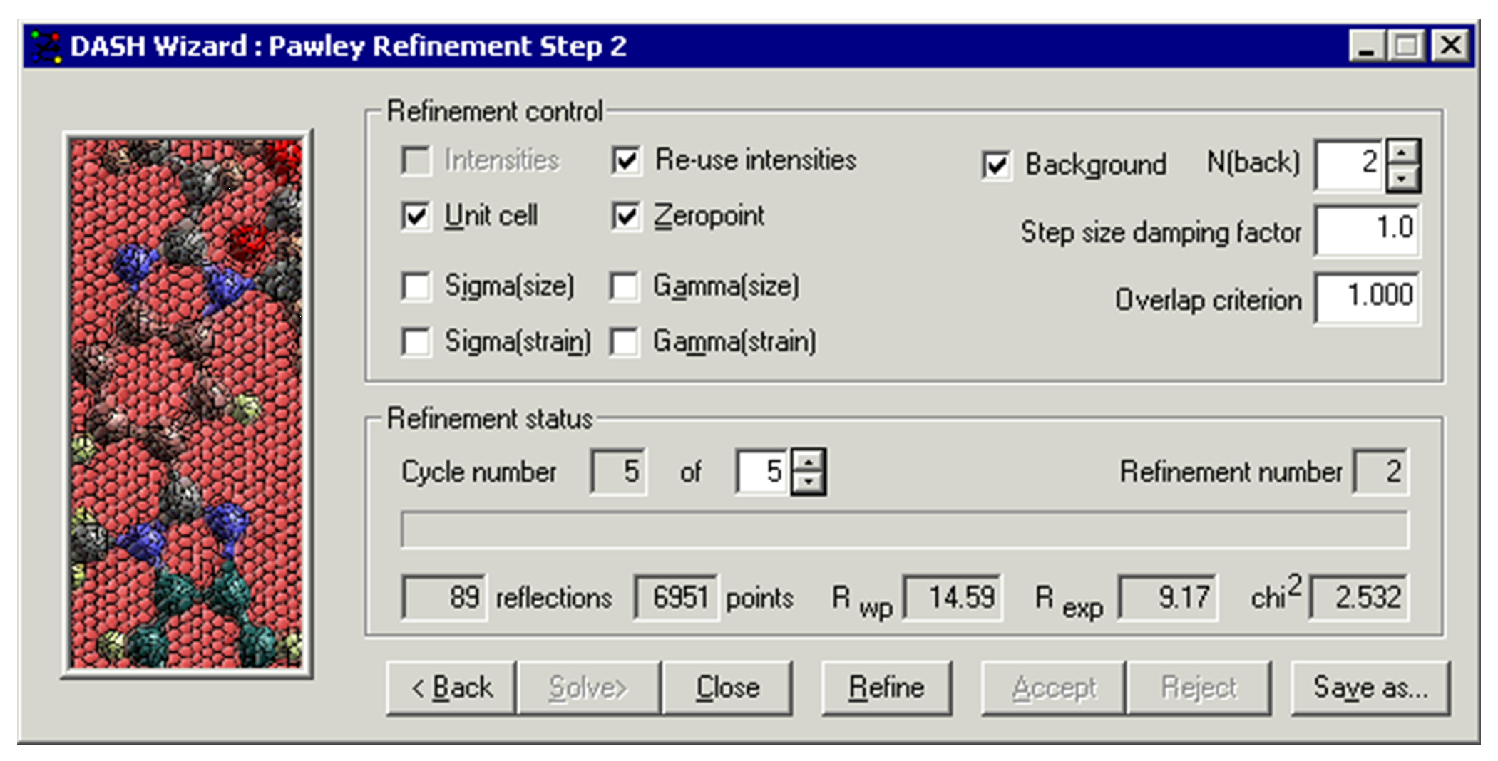
Using the Example.xye file, the unit cell parameters and space group information, and having selected 8 peaks (see Picking of Peaks for Pawley Refinement) you will arrive at a window as shown in the Pawley Refinement Interface.

• In this example, we have assumed that the background has been fitted by the Monte Carlobackground subtraction routine. If the background had not already been subtracted, the only difference would be that N(back) would be automatically set to 10.

• The data has been truncated to a resolution of 2.0 Å.

• In the initial Pawley refinement, only the terms describing the background and the terms corresponding to individual reflection intensities are refined, using the previously refined unit cell and zero-point.

• When you select Refine 3 cycles of least squares are performed.

• This should return figures similar to the ones given below:

  89 reflections 6950 points R_wp= 33.52 R_exp = 9.22 χ² = 13.210

• Select Accept to accept the results of this refinement, the fit is displayed.

• Now click in the main window and select Home to see how well the data are fitted. The (observed minus calculated) plot is shown in pink and emphasises any misfit in the data. If you look closely at the data, you are likely to see something like this:

The next stage is to refine Background, Intensities, Unit Cell and Zeropoint. DASH assumes that after the initial background and intensities fit, you will automatically want to refine the unit cell and zero-point. Accordingly, tick marks are automatically set in the menu boxes. Normally 5 cycles of refinement are sufficient. Click the Refine button and then the Accept button to store the results of refinement. The Pawley Refinement Status window now looks like this:

Saving the Results of Pawley Refinement (Pawley-Fit files)

• In the example shown in Pawley Refinement: an Example the ² of 3.087 is very good, so you would then save the results of this refinement as the basis for structure solution.

• Select Accept and then Save as...; the Save Diffraction Information for structure solution window appears into which you can enter a file name, e.g. Example.sdi; click Save.

• You can save the results of several independent Pawley refinements, each in its own Pawley-Fit file, with extension .sdi.

Mathematical Problems with Pawley Refinement

For poor quality data sets there can be problems in fitting the background with the polynomial mathematical procedure. When this happens an Errors detected during Pawley fit window will appear:

View fit list file shows the output of the fitting program. If you look at the last few lines of this file there are messages as to why the procedure failed. Do not accept the results of this refinement. Check the following:

• 2θ range: consider if there is really any useful data above a certain 2θ, and truncate (see Truncating the Data).

• Overlap Criterion: it is always worthwhile re-running the refinement with a larger value of the Overlap Criterion (see Pawley Refinement Interface). For heavily overlapped, weak data, a value of 2.0 may suffice to stabilise the refinement.

Truncating the Data

• DASH limits the number of reflections that can be refined in a Pawley refinement to around 350. This is all that you will need to solve the majority of organic structures. Accordingly, it may be necessary to truncate the data, i.e. throw away counts above a certain 2θ value.

• The actual truncation of the data must be done before the Pawley refinement stage, either by manually editing the input data file or by using the Wizard.

• You must judge the point in the profile at which the significant information ends.

• As a general rule, if data can be used up to 1.5 Å, there will generally be enough information to solve most organic structures; i.e. for CuK_α1 radiation (wavelength l = 1.54056 Å):

  θ = sin-1(l/2d)
  Therefore:
   θ = sin-1(1.54056/ (2 * 1.5) ) ≅ 30^o
  Therefore:
  2θ ≅ 60^o
  
  Sometimes, the powder pattern will not contain useful data to this high angle. In such cases, it is better to cut the data down to lower resolution e.g. 2.0 Å or even 2.5 Å.

• Examples are provided illustrating some suitable cut-off points for:

• A high resolution profile (see Truncating High Resolution Data: an Example).

• A medium resolution profile (see Truncating Medium Resolution Data: an Example).

• A low resolution profile (see Truncating Low Resolution Data: an Example).

Truncating High Resolution Data: an Example

• Synchrotron dataset, with an incident wavelength of 1.1 Å; thus data were collected to maximum 2θ = 60^o, equating to 1.1 Å spatial resolution:

• There are 418 reflections in this data range, which is slightly more than DASH will handle by default. However, a significant proportion (nearly 25%) of these reflections occur in the last 5% of data:

• Although the crystal is still diffracting quite strongly at this point (sufficiently well for the information content to be useful in structure refinement) it is clear that the extent of reflection overlap is high. If we cut the data limit back 5^o to 55^o, we simplify the problem by reducing the number of reflections to be refined to only 323, at the cost of only 0.1 Å loss in spatial resolution. In fact, this structure can easily be solved from data extending to 1.0 Å resolution (43^o 2θ) and the total number of reflections in this range is then only 163.

Truncating Medium Resolution Data: an Example

• Synchrotron dataset with an incident wavelength of 0.85 Å, so 1.5 Å resolution equates to around 2θ = 33^o:

• It is clear that diffraction is still strong at the high-angle end:

• There are around 350 reflections in the full data range and this can easily be fitted, so truncation is not necessary.

Truncating Low Resolution Data: an Example

• Synchrotron dataset with an incident wavelength of 1.15 Å; thus, 1.5 Å spatial resolution equates to a 2θ value of 45^o. However, it is clear that the diffraction data is fading long before this point:

• Given the poor signal to noise ratio, there is little point in fitting the data beyond about 30^o, which equates to about 2.2 Å resolution. (This is sufficient to solve the structure.)

Choosing Peaks Prior to Initial Pawley Fitting

The first step in Pawley fitting is to select some peaks for refining the peak-shape parameters and the unit cell dimensions. Once enough peaks have been selected (usually 8 to 10), and stable estimates of these parameters have been obtained, an initial Pawley refinement of the background and reflection intensities can be performed. Guidelines for peak selection are:

• If possible, choose strong, well-defined reflections that, collectively, span a broad 2θ range.

• They should include at least one or two peaks at low 2θ, so that any low-angle peak asymmetry is well described in the refinement of the peak-shape parameters.

• If possible, isolated reflections should be chosen. These can be identified by looking at the tick marks at the top of the display, which show the reflection positions calculated from the cell and space group you have specified. However, it is valid to fit multiple peaks if necessary.

• As selection of peaks proceeds, DASH will update peak shape parameters, and then cell parameters, and then indicate that it is ready to perform the initial Pawley refinement.

Choosing Peaks Prior to Initial Pawley Fitting: an Example

The following example of peak selection for Pawley refinement illustrates some of the situations you will encounter:

• Fitting the first three peaks in the pattern. These peaks are all fairly strong and well separated and can be fitted easily. Inclusion of these peaks helps subsequent cell refinement (as they correspond to low order reflections) and gives a good parameterisation of any asymmetry present:

• Looking further up the pattern, there is a strong peak that could be selected, but it has a weak satellite peak to the right, which would need to be fitted simultaneously. The weak peak is not strong enough to provide useful peak parameterisation information in its own right, but it is strong enough to affect parameterisation of the strong peak, so would have to be included in the fit. There are almost certainly better choices at other points in the pattern, so do not use these peaks:

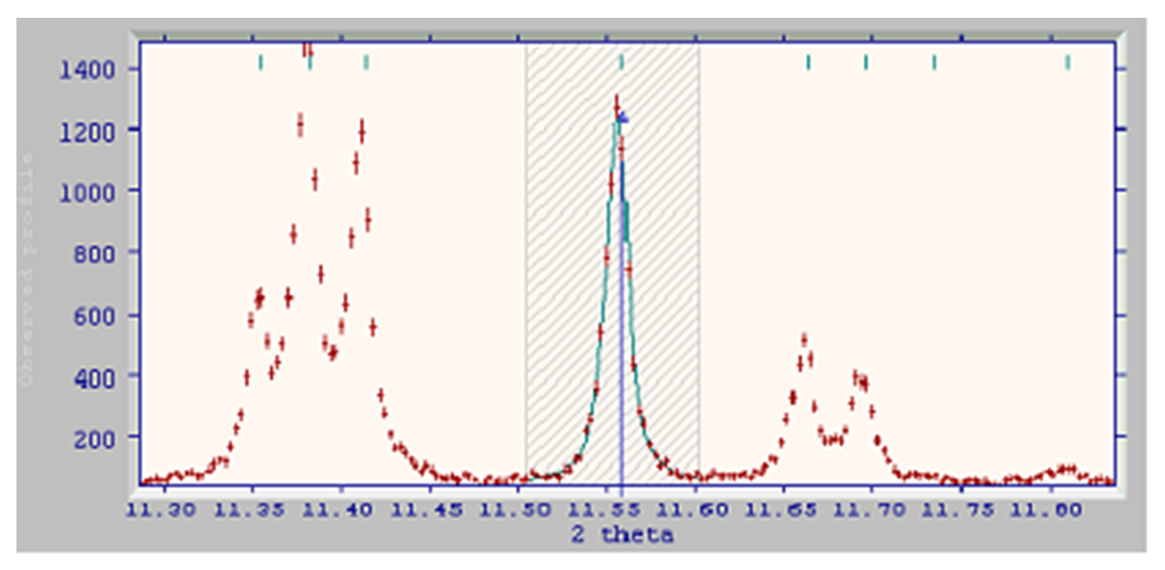
• Still further up the pattern, there is a strong isolated peak that can easily be used. The triplet and the doublet on either side of it could be selected too, but we really want to sample peaks throughout the 2θ range in order to parameterise the peak shape right across the pattern. By fitting the triplet, we simply get three peaks telling us about the local peak shape around 2θ = 11.37^o. Fitting the single peak at ~11.56^o gives us exactly the same information:

• Even further up the pattern, there is a nicely isolated pair of fairly strong peaks. We could fit these reflections individually, but as they overlap a little, it is better to fit them together as a doublet:

• Note that these two peaks contribute two entries in the list of peak positions (select Peak Positions from the View menu) yet only a single entry in the lists of peak shape parameters (select Peak Widths from the View menu) as both peaks have been fitted with the same values for sigma and gamma.

• Moving further up again, there is a peak that has contributions from two Bragg reflections (i.e. there are two tick-marks close together above the peak), but there are no clues as to their exact relative positions. Peaks such as this are best avoided because, each time a peak is fitted, DASH attempts to refine the input unit cell (the one you obtained by indexing, and entered at the start of the Pawley fitting process). In this situation, the peak positions are not well defined and there is a risk that the cell could be refined away from the correct values. Thus, avoid:

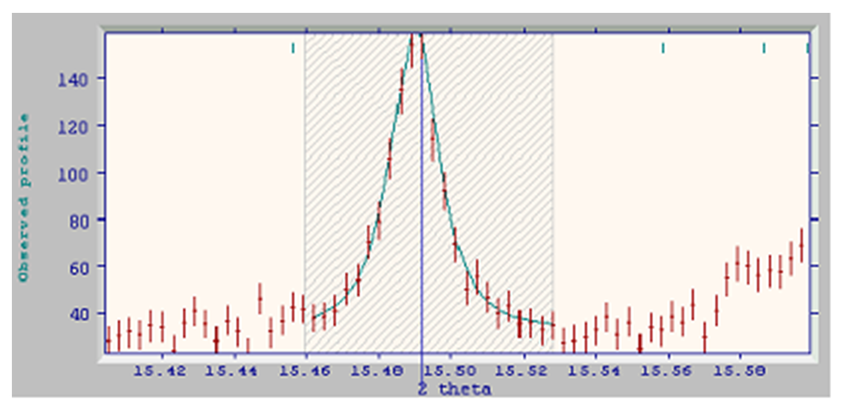
• Next, we find a moderately strong reflection which is sufficiently isolated to allow fitting, even with a narrow selection range. The very weak peak on the left is not strong enough to interfere:

• This is the 7^th peak selected; thus we have accurate peak shape descriptors and peak positions for 7 peaks throughout the pattern. This is sufficient information for a least-squares cell refinement to be performed on this monoclinic cell, and DASH will do this automatically. A sign that lattice parameter refinement has commenced is that the tick mark above the peak jumps closer to the peak after fitting; this indicates that the cell has been updated to incorporate the latest peak position.

• DASH has automatic settings that determine the best point at which to attempt a full Pawley refinement. At this time, it automatically displays the Pawley Refinement Status window. In this example, the window is not yet displayed, so we continue picking peaks.

• Further up the pattern, there is another isolated peak which is easily fitted. Now, with a total of 8 peaks fitted, the Pawley Refinement Status window is displayed automatically.

Initial Pawley Fitting of Intensities and Background

• Once enough peaks have been selected and the program has stable estimates of the cell dimensions and peak-shape parameters, you can perform an initial Pawley fit of the reflection intensities and the background. This will be indicated by the appearance of a pop-up window.

• Usually, you should keep the cell dimensions and peak-shape parameters fixed in this initial refinement. Allowing them to vary is likely to destabilise the refinement.

• The following subsections cover:

• Background fitting (see Background Fitting of Raw Data in the Pawley Refinement).

• Reflection-intensity fitting (see Reflection-Intensity Fitting).

Background Fitting of Raw Data in the Pawley Refinement

• Note that in this example, we have assumed that the background has not been fitted by the Monte Carlo background subtraction routine. This is by way of illustrating use of the Pawley refinement for a raw data set.

• Background intensity is primarily due to amorphous content in the sample and scattering from experimental components such as a glass capillary or cryostat chamber.

• The background is fitted to a polynomial which, by default, has 10 terms.

• It is undesirable to use more background terms than necessary to describe the data, since high order polynomials can begin modelling genuine peak intensity. This leads to high correlations between the background and peak intensities, especially at high angles.

• A polynomial with as few as 5 terms might be enough for a flat or gently curving background; at the other extreme, you should never have to use more than about 15. Normally, the simplest policy is to try the default of 10 and accept it if the fit looks satisfactory.

• The following example profile has a very non-uniform background:

• In this case, a total of 10 background terms were used and the Pawley fit returned R_wp=5.9, R_exp=2.5 and ² = 5.6. Some misfit (though not much) is evident between the peaks at high angles:

• Increasing the number of background terms to 15 brings about a significant improvement, with R_wp=5.65, R_exp=2.5 and ² = 5.15:

• A further increase to 20 background terms improves the fit slightly, but the high angle plot is virtually indistinguishable from that with 15 parameters, so the gains in going to 20^th order are not worth it (In fact, the fit with a 10^th order polynomial is sufficient to solve the structure).

Reflection-Intensity Fitting

• In fitting the individual reflection intensities, a peak shape description function is centred at the calculated 2θ of each reflection. The parameters used in the function (₁, ₂, ₁, ₂) have already been determined from the initial set of peaks you selected and should not be varied at this stage. They can be refined later, once the unit cell and zero-point have been fully optimised.

• The fitting procedure not only estimates the individual reflection intensities but also their covariances.

• If a group of reflections are too close together, then the observed intensity for that clump of reflections is treated as a single variable, with the resultant intensity partitioned equally between the component reflections.

• Look at the output file polyp.lis to get information about which reflections have been merged together in this way. The file also lists the total number of reflections and other diagnostic information.

Hints for Improving the Pawley Fit

Once a reasonable initial Pawley fit has been obtained, it can usually be improved by:

• Adding into the refinement the cell dimensions and zero-point (see Cell Dimension and Zero-Point Refinement).

• Refining some or all of the peak-shape parameters (see Peak Shape Refinement).

Cell Dimension and Zero-Point Refinement

An initial Pawley fit can almost always be improved by adding into the refinement the cell dimensions and zero-point.

• The cell dimensions will now be refined against the whole of the profile rather than the small number of peaks you chose initially.

• The zero-point (origin of 2θ axis) may have been measured experimentally for the instrument on which data were collected, but it is always desirable to refine it anyway. A refined absolute value of 0.01^o would not be atypical.

• An error in the zero-point may manifest itself on the profile difference plot by a systematic shift in peak positions.

Peak Shape Refinement

• Unless and until the peak-shape parameters are explicitly included in the Pawley refinement, their values will be based only on the few peaks you chose when setting up the initial refinement.

• Normally, you should not need to refine the peak shapes further. However, if you notice that certain peaks are not well fitted, it may be worth including them directly in the peak shape estimation process. Sweep out an area to select the peak and fit as before. The overall peak shape description will be updated and you can re-run the Pawley fit with the updated parameters.

• The peak shape used within DASH is a full Voigt function (a convolution of a Lorentzian and a Gaussian function) which uses 2 parameters (₁ and ₂) to describe the angle-dependent Gaussian component:
  ² = ₁² sec²  + ₂² tan² 

  and 2 parameters (₁ and ₂) to describe the angle-dependent Lorentzian component:
   = ₁ sec  + ₂ tan 

  There are also two asymmetry parameters, HPSL and HMSL, but these are fully defined by the peak fitting procedure and cannot be refined during the Pawley fitting.

• The refined values of the peak-shape parameters may be seen by selecting Peak Widths from the View menu. The values should all be positive, though small negative values are occasionally obtained.

• There may be some cases (usually those that involve some anisotropic line broadening) in which it is useful to refine the peak parameters within the least squares of the Pawley fit. In general, only peak shape parameters of sizeable magnitude should be refined; there is little to be gained by refining a single parameter that is very close to zero, as its contribution to the overall magnitude of the composite width will be negligible. Refinement of small peak shape parameters may lead to numerical instabilities.

Assessing the Quality of the Pawley Fit

The quality of a Pawley fit must be judged in two different ways, both of which are important:

• How good are the goodness-of-fit parameters? (see Interpreting Pawley Fit Parameters)

• How do the observed and fitted profiles compare visually? (see Visual Assessment of Pawley Fit)

Interpreting Pawley Fit Parameters

• The parameters R_wp, R_exp and ² are a guide to the quality of a Pawley fit (see Appendix D: Definitions of DASH Figures of Merit).

• Ideally, R_wp should be close to R_exp and ² should be close to 1.0.

• However, this ideal is often not met in practice, particularly before the cell and zero-point have been refined, and particularly with laboratory data. For example, four recent Pawley fits in a laboratory gave ² values of about 1, 5, 15 and 30. These were all synchrotron data sets; generally you should expect higher ² values with laboratory data.

• A ² < 1.0 indicates that the ESDs on the data set are not quite correct (specifically, they have been overestimated).

• You should not rely solely on the fit parameters; visual inspection of the fit is essential.

Visual Assessment of Pawley Fit

• There is no substitute for examining by eye the fit of observed and calculated profiles; figures of merit which pertain to the entire pattern do not highlight local problems, such as peaks that might not be fitted at all (e.g. impurity peaks).

• The following example shows a good fit. The pink difference plot shows no marked areas of misfit:

• Zooming in on the fit to the data in the mid-range of the pattern shows an excellent fit to the data:

• The same is true at high angle:

• If the positions of calculated and observed peaks do not match well (e.g. because the zero-point and unit cell are not properly refined), there is a characteristic sinusoidal difference plot:

• In this example, the problem is solved by refining the cell and zero-point:

• Slightly too narrow peak widths result in a rise; dip; rise difference plot. This is often seen as a weak trace around very strong peaks:

• A small misfit in tails is not serious: you should start to worry if the misfit is somewhere approaches one-third of the peak height.

• If a dip; rise; dip difference signature is seen, the calculated peak is too wide.

Numerical Instability in Pawley Refinement

Sometimes, a Pawley refinement will diverge and DASH will display an error message. Possible ways of removing the numerical instability include:

• Truncating the data a bit more (see Truncating the Data).

• Reducing the number of background parameters.

• Taking advantage of the automatic background subtraction that DASH offers (see Removing the Background from Diffraction Data).