StructureSolution

Structure Solution

Overview of Structure Solution

DASH solves structures by altering the positions, orientations and (where appropriate) conformations of the molecules in the unit cell, subject to the constraints of space group symmetry, until a good match is obtained between calculated and observed intensities. This process is a search for a global minimum in a multi-dimensional parameter space, the parameters being positions, rotations (expressed as quaternions) and torsion angles. This search is performed using a simulated annealing algorithm. This section covers:

• The basics of simulated annealing (see Fundamentals of Simulated Annealing).

• Using the interface for structure solution (see Using the Interface for Structure Solution).

• Simulated annealing parameters (see Simulated Annealing Parameters).

• Monitoring the progress of structure solution (see Monitoring the Progress of Structure Solution).

• Assessing the final answer (see Assessing the Solution).

• Troubleshooting (see Things to Try When Structure Solution Fails).

• Final Rietveld refinement (see Final Rietveld Refinement).

• Limitations of DASH (see DASH Limitations).

Fundamentals of Simulated Annealing

• The algorithm starts by assigning random values to the parameters (molecular position, orientation and conformation).

• Agreement between calculated and observed (Pawley) intensities is assessed by computing a ² goodness-of-fit statistic.

• One of the parameters is randomly altered and the ² value recalculated.

• The algorithm accepts the new parameter value if the ² value has gone down (i.e. the fit has been improved). If the ² value has gone up, then the new value is either rejected or accepted, subject to a Boltzmann distribution. The probability of accepting such an uphill move depends on the current temperature of the system; the higher the temperature, the more likely it is that an uphill move will be accepted.

• This procedure is repeated many times, each parameter being altered in turn.

• At the end of a predetermined set of moves, the temperature is lowered, thus decreasing the chances of acceptance of uphill moves; the above process is then repeated.

• The algorithm terminates when the system converges to a minimum (hopefully, global) in ² space, or when a maximum number of moves is reached.

In essence, the algorithm tries to move downhill in ² space, but occasionally allows uphill moves in order to let the system escape from local minima.

Using the Interface for Structure Solution

In order to use the interface for structure solution you can either:

• Call the Wizard by clicking on the following icon:

• Either select Simulated Annealing Structure Solution

• Or select Structure Solution from the top-level Mode menu

• Or click on the following icon:

This will bring up the DASH Wizard : Molecular Z-Matrices window, shown below, which you can use to:

• Input Z-matrices (see Input of the Z-Matrices).

• Edit Z-matrices (see Editing a Z-Matrix).

• Edit Z-matrix rotations (see Editing Z-Matrix Rotations).

• Look at preferred orientation (see Preferred Orientation).

• Check and set parameter ranges (see Checking and Setting Parameter Ranges).

• Access Mogul, if available, via the Parameter Bounds window (see Using DASH with Mogul).

• Start the simulated annealing run (see

• Starting the Simulated Annealing Run).

• Select the Pawley-Fit file, with extension .sdi, saved after the Pawley refinement. Either type in the file name, or browse for files with extension .sdi.

• The main window now displays the diffraction data with tick marks.

• Proceed to input Z-matrix files for the molecule(s) (see Input of the Z-Matrices).

Input of the Z-Matrices

• Click on the icon. This will display all files available with the extension .zmatrix, .mol2, .mol, .ml2, .pdb, .cssr, .cif or .res.

• Select the file and click Open.

• When a Z-matrix file is successfully read in the number of parameters set up is displayed to the right of the open-folder button. The first molecule should show that at least 6 parameters are created. Each rotatable torsion angle adds 1 to the total parameters.

• If there is more than one molecule in the asymmetric unit, repeat the loading process for the next Z-matrix file.

• Select View to view a Z-matrix. Flexible torsion angles can be colour coded by ticking the Colour flexible torsions check box under Options | Configuration...

• Select Edit... to edit a Z-matrix (see Editing a Z-Matrix).

• Click on the icon to clear a Z-matrix you have loaded but do not want to use.

• Then click Next > (see Checking and Setting Parameter Ranges).

Atom Tethering

• DASH features the ability to apply tethers between unassociated atoms in the solution process. The main function for atom tethering is to allow a user to break a ring in a molecule to make it flexible. A tether can then be used to make the code force ring closure while allowing the rings internal torsion angles to vary.

• The intensity ²is biased by the tether: two atoms A and B are separated by a distance of d_AB. If the ideal distance of separation is d_ideal and there is a permitted tolerance of t then the modified ² is given by:

² = ² + qW (MAX(0.0,[|d_ideal - d_AB| -t]) ²

• Where W is a user supplied weight, and q is an annealing factor: the annealing factor scales linearly from 0 to 1 as the simulated annealing progresses.

• It is also possible to tether atoms in different Z-matrices to one another, to allow the user to input information regarding the presence of a given interaction.

• Atom tethering of independent Z-matrices will rarely improve the success rate of the solution search for good quality data, and in certain cases may even degredate performance due to the addition of barriers into the Monte Carlo search process, but may be useful with poorer patterns where there is higher uncertainty in the reflection intensities.

• To use, click the Set Fragment Restraints button in the Parameter Bounds window.

• This will launch a dialogue: The user can select atoms from each fragment and a separation distance between them for 1 or more pairs of atoms, either within a single fragment or between fragments. The user here also specifies the ideal distance between the pair of fragment atoms. A default weight is specified as 100.0.

Editing a Z-Matrix

This window allows various atomic properties to be modified:

• The list of atoms displayed allows you to delete individual atoms from the Z-matrix and allows you to change the label, element, Biso and occupancy of each individual atom.

• Bisos and occupancies can be changed for groups of atoms using the Set button.

• Re-order re-orders the atoms carbon atoms first, followed by the remaining elements in alphabetical order, and hydrogen atoms last.

• Re-label re-labels the atoms as element + sequential number, e.g. C7 and Br24.

• Rotations... displays the Edit rotations / Z-matrix dialogue box (see Editing Z-Matrix Rotations).

• Save As... allows saving of the edited Z-matrix with a new name.

• View displays the edited Z-matrix.

• Save saves the edited Z-matrix.

• OK returns you to the DASH Wizard : Molecular Z-Matrices window, keeping all changes. If atoms have been deleted, DASH will try to assemble a new Z-matrix from the remaining atoms.

• Cancel returns you to the DASH Wizard : Molecular Z-Matrices window, discarding all changes.

Editing Z-Matrix Rotations

This window allows full control over the way orientations of a Z-matrix are handled during simulated annealing. It is recommended that the .sdi file has been loaded first, so that the unit-cell parameters are available for visualisation of the centre of rotation and the initial orientation:

• The origin of rotation can be specified in the same manner as in the .zmatrix file (see Molecule Translation and Rotation; Special Positions) and can be checked visually by pressing View and switching on the display of the cell-axes in your viewer. When using Mercury, select Show cell axes (lower right) rather than Packing (lower left).

• The rotations of molecules that lie on a rotation axis or in a mirror plane can be restricted to that rotation axis or to the axis perpendicular to the mirror plane. When restricting rotations to a single axis, the initial orientation of the molecule with respect to the unit cell needs to be specified. This can be done by entering the Euler angles or quaternions.

• If the axis of rotation is specified either as the line through two atoms or as the normal to the plane defined by three atoms (i.e. if the axis of rotation can be specified from the molecule alone) it is also possible to choose the initial orientation such that the axis of rotation is aligned with an axis specified in fractional coordinates. The initial orientation can be checked by pressing View and switching on the display of the cell-axes in your viewer. When using Mercury, select Show cell axes (lower right) rather than Packing (lower left).

The single axis of rotation is specified by the origin of rotation of the molecule and one other vector, which can be any of the following:

• The vector between two atoms. Just enter the numbers of the atoms. To easily establish an atom’s number, re-label the atoms first using Re-label and then display the atom labels in Mercury.

• Fractional co-ordinates, e.g., 0,0,1 would restrict the rotation of the molecule to be parallel to the c-axis.

• Normal to a plane defined by three atoms in the molecule. Just enter the numbers of the atoms. To easily determine the atom’s number (or atom ID), re-label the atoms first using Re-label in the previous screen and then display the atom labels in Mercury.

• OK returns you to the Edit Atomic Properties / Z-Matrix window, keeping the changes that have been made. Note that clicking Cancel in the Edit Atomic Properties / Z-Matrix window will also cancel changes made in the Edit rotations / Z-Matrix window.

• Cancel returns you to the Edit Atomic Properties / Z-Matrix window, discarding the changes that have been made.

• View displays the Z-matrix. The unit-cell axes are included, allowing you to check the origin and initial orientation of the molecule. To display the unit-cell axes when using Mercury, select Show cell axes (lower right) rather than Packing (lower left).

Preferred Orientation

The March-Dollase preferred orientation correction can be used. The direction of the preferred orientation must be entered in this window, the magnitude is optimised during the simulated annealing. All preferred orientation parameters are written out to all molecular output files.

Checking and Setting Parameter Ranges

You arrive at the DASH Wizard : Parameter Bounds window after loading the Z-matrix files (see Input of the Z-Matrices).

• The purpose of the menu is to allow you to control which parameters are variable or fixed. Each parameter has a starting value, a lower limit and an upper limit. The box F is ticked for fixed or un-ticked for variable parameter control respectively.

• If the Randomise initial values check box is selected, the starting values for the parameters that are varied during the simulated annealing step will be set to random values before starting the simulated annealing. When Randomise initial values is not selected, the values shown in this dialogue window will be used, allowing a previous run to be restarted where it left off. (If the first simulated annealing cycle is a dummy cycle to determine the initial temperature, the values will be reset at the start of the second cycle.)

• Set any of the molecular translation parameters x(Frag1), y(Frag1), z(Frag1) as fixed by clicking F-box if required by the space group e.g. in P2₁ we can fix the y-translation for the first molecule given.

• Generally it is not necessary to fix any of the molecular rotation parameters Q0, Q1, Q2, Q3.

• Torsion angles are not normally fixed, and will have a range of 360^o. However, upper and lower bounds can be entered here to define a single torsion angle range to be searched.

Starting the Simulated Annealing Run

You will reach the DASH Wizard : Simulated Annealing Protocol window from the parameter range menu (see Checking and Setting Parameter Ranges).

This allows the user to set the variables that control the simulated annealing run.

• Default Simulated Annealing values are provided which are usually satisfactory, the default values from DASH 3.3.7 onwards are labelled as Kabova (2017) referring to the relevant publication on optimisation of the SA parameters (for more details, see Optimisation of simulated annealing parameters). For reference back to previous studies, the older default values are still available by clicking on the v3.3 Defaults button. To accept these values simply click the Next > button (see Starting the Simulated Annealing Run). The meaning of these parameters is discussed in Simulated Annealing Parameters.

• Maximum number of SA runs: the default setting is 10 runs. It is generally advisable to try several SA runs using different random number seeds; this is done for you automatically if you specify the number here. The best solution from each run is stored in suitably numbered files (see Files saved from multiple runs of SA).

• Maximum number of moves per run: the default setting is 10,000,000. When this number of moves is reached, the run is terminated, whatever the value of ² (see Convergence Criteria).

• Profile chi-squared multiplier: the default setting is 5.0. This means that if the SA profile χ² falls below a value 5.0 times that of the Pawley-fit ², and the minimum number of moves has been exceeded, the run is terminated (see Convergence Criteria).

• The Print... button will pop up a text editor window containing a summary of the current simulated annealing parameters. This text file can be edited, saved and printed.

Setting Torsion angle ranges

Manually entering torsion angle ranges

• Torsion angles are not normally fixed, and will have a range of 360^o. However upper and lower bounds can be entered here to define a single torsion angle range to be searched such as -10 to 10^o. If DASH has access to Mogul, appropriate torsion angle ranges can be explored by hitting the Modal button (see Using DASH with Mogul). Mogul is a molecular geometry database which forms part of the CSD Portfolio and is available separately from the CCDC. If Mogul is not accessible, modal torsion angle ranges can be defined in the Modal Torsion Angle Ranges dialogue that will appear on hitting the Modal button.

• The Modal Torsion Angle Ranges dialogue box allows bimodal and trimodal torsion angle ranges to be defined. The radio buttons at the top of the dialogue box are used to choose whether bimodal or trimodal torsion angle ranges are required.

• In the boxes labelled Upper and Lower enter the upper and lower bounds of a single torsion angle range, thus if a bimodal search of the torsion angle space of 30 - 90^o and -30 to -90^o is required, enter 30.0 in the Lower box and 90.0 in the Upper box. The complementary range is automatically determined and displayed. Torsion angles within both of the displayed ranges will be generated during the simulated annealing run. Planar torsion angle ranges (centred around 0^o and 180^o) can be searched by defining a bimodal range such as -20^o to 20^o. The complementary range determined and displayed will be -160^o to 160^o. If a trimodal range is chosen then torsion angles will be sampled from the defined space and two further ranges at +/- 120^o.

• To accept the defined torsion angle ranges, press OK. This will return you to the main Parameter Bounds dialogue box, and the torsion angle to which modal ranges have been applied will be highlighted in red.

• Hitting Cancel will result in all edits, since the last accepted modal range, being ignored.

• Hitting Non Modal will return you to the Parameter Bounds dialogue box and the full 360^o torsion angle range will be applied. A non-modal torsion angle range is shown in black.

• Torsion angles may be fixed at a value. Click the F-box, and then type in the required value in the initial box e.g. 0.0

• When all parameter ranges are set, click Next > (see

• Starting the Simulated Annealing Run).

Using DASH with Mogul

• If DASH has access to Mogul, appropriate torsion angle ranges can be explored using this program. Mogul is a molecular geometry database which forms part of the CSD Portfolio and is available separately from the CCDC. If Mogul has been installed in the default location, DASH should automatically find the path to the executable and this path will be displayed in the Configuration window (see Configuration). However, if DASH does not find the path to the Mogul executable it is possible to enter a path to Mogul in the Configuration window.

• Once a path to Mogul is present in the Configuration window, hitting the Modal button will launch Mogul and a histogram of the distribution of angles obtained from structures within the CSD for the chosen torsion angle will be displayed. It should be noted that the Mogul histogram displays all torsion angles, positive and negative on a positive axes, i.e. 0-180. The structures that contribute data to the histogram can be examined by clicking on the View Structures tab in the Mogul window.

• Upon closing the Mogul window the Modal Torsion Angle Ranges dialogue will be displayed and, if the torsion angle had a distribution that DASH recognised, a recommended range of torsion angle values will be shown in the Upper and Lower sample range boxes. It is recommended that the user check that the suggested ranges are appropriate before accepting them. The lower and upper bounds on the ranges can be edited if different ranges are thought to be more suitable.

• To accept the defined torsion angle ranges, press OK. This will return you to the main Parameter Bounds dialogue box, and the torsion angle to which the modal ranges have been applied will be highlighted in red.

• Hitting Cancel will result in all edits, since the last accepted modal range, being ignored.

• Hitting the Non Modal button will return you to the Parameter Bounds dialogue box and the full 360 torsion angle range will be applied. A non-modal torsion angle range is shown in black.

Mogul Data Biasing

• Mogul data biasing (MDB) is an alternative way of using Mogul to improve retrieval of correct answers in searching. MDB uses Mogul distributions to bias the sampling in searching to tend to favour regions of space where Mogul indicates there is a high likelihood.

• The underlying code works by modifying the Maxwellian distribution used for each step. In simulated annealing, each trial move is calculated by first taking a number at random from a maxwellian distribution: The Maxwellian tends to favour particular moves dependent on the current annealing temperature. In MDB, the Maxwellian distribution is modified to favour moves to torsion angles into regions of space that are heavily populated in the corresponding Mogul distribution.

• This is summarised below. The Maxwellian is binned and multiplied by the respective bin in the mogul (The mogul distributions are first modified so that no bin contains zero hits; this ensures that no parameter space is completely excluded from the Maxwellian).

• MDB can have benefit, but on occasion can detract from the solution process. By using MDB, the user is assuming that the torsion angles in the correct solution lie within the most commonly observed ranges of torsion angles. In some structures, this clearly will not be the case; in such situations MDB will tend to bias the search algorithm away from the correct answer. Tactically, it is best to use MDB in initial runs. If, however, the structure fails to solve, still consider re-running the solution SA without MDB as a fall back, in case your structure contains an unusual torsion angle.

• The drawbacks are mercifully rare: MDB has a beneficial effect in > 90% of the test cases that we use it for, either in speeding up the search by reaching the global minimum more quickly. In some large structures we find that MDB makes the solution process succeed in more runs than without MDB.

• MDB can be enabled by clicking the Set MDB button in the Parameter Bounds wizard window. The choice of distributions to use can be controlled by increasing or decreasing the minimum hits; the higher the number of hits, the more populated a mogul distribution has to be to be used in MDB. The default of 10 observations may seem a little low: Note, however, that due to the nature of the algorithm used, using distributions with low numbers of observations in fact makes little difference to the solution process, as the weight of bias to the Maxwellian distribution is in proportion to the number of hits in the distribution. A distribution with only 10 observations in will not really change the sampling for a given torsion by a great amount.

• DASH also supports reading SA input settings directly from DBF files. This, in principle, could allow the user to set up searches with data distributions from other sources. A given torsion angle can be biased by specifying a parameter and range for the given torsion in the input DBF file in the following form:

-65.95955 MDB -180.00000 180.00000 18 0 0 0 0 2 7 10 5 0 0 0 0 0 0 0 0 2 14

Here, the parameter's start value is first, followed by the control keyword 'MDB'. Subsequently we have the maximum and minimum value range for the parameter followed by the number of bins in the associated histogram. Finally we have the histogram itself. Clearly the histogram could easily be altered to reflect, say, the range of torsion angles observed in a conformational analysis for the associated molecule.

Simulated Annealing Parameters

Optimisation of simulated annealing parameters

• The default simulated annealing parameters available in DASH are the result of a focused research study to optimise the values of three key parameters. This process improved the success rate in finding the global minimum by an order of magnitude using a test sets of over 100 powder diffraction datasets compared to the previous default values.

• For more details, see the Kabova et al., 2017 paper referred to in Appendix I: References.

Starting Temperature

• If the search space is complex (i.e. contains many local minima), the starting temperature must be high so that the algorithm will make many uphill moves in the early stages. This will ensure that the search space is explored thoroughly.

• Setting T0 to zero in the interface instructs DASH to select the starting temperature automatically. This is recommended, at least in the first simulated annealing run, until you get a feel for the problem.

• DASH selects the starting temperature by performing a brief simulated annealing run at high temperature and monitoring the variance of the ² value as random moves are made in parameter space. Based on the results, the starting temperature is set to a value that will allow the algorithm to escape deep local minima at the outset of the search (i.e. the higher the variance in ², the higher the starting temperature).

• The optimum starting temperature is very data dependent; it could be 25 K in a good case (a simple response surface with few local minima), but much higher (>1000 K) for a complex problem.

Cooling Rate

• DASH typically uses a fixed, conservative cooling rate of 0.270 K (i.e. the rate at which the temperature is reduced) for the annealing process. The temperature reduction is applied at the end of each cycle of annealing.

• The cooling rate is not constant as the annealing proceeds. If DASH detects large fluctuations in ² (implying that the algorithm is in an interesting region of parameter space) it automatically reduces the cooling rate to ensure a thorough search.

• The slower the cooling rate, the more thorough the search of parameter space and the greater the chances of finding the global minimum. However, a slow cool obviously takes longer.

Number of Moves

The values of N1 and N2 determine the number of moves (random parameter changes) that are made at each temperature. Specifically, if there are N variable parameters (positional, rotational, conformational), the simulated annealing performs N1*N2*N moves at each temperature. Default values are N1 = 73 and N2 = 56; these will only need to be increased in difficult cases.

Convergence Criteria

How does DASH know when it has a correct answer, and thus when to stop the annealing process? The ² obtained from the Pawley fit represents very much the best fit that can be obtained from the data (all intensities are treated as being variables in the least-squares process) and so if DASH comes close to achieving this profile ² in the annealing process, there is a good chance that the answer is correct.

There are a number of reasons as to why you will not obtain as good a fit in the structure solution process as you did with the Pawley fit:

• Your input model is based on a number of chemical assumptions, some of which may not be entirely accurate.

• The assumption is that all non-H atoms have fixed temperature factors.

• There may be some preferred orientation in the sample.

Accordingly, DASH realises that if the profile ² comes within a preset multiple (default value = 5.0) of the Pawley ², then there is a good probability that this structure is worth examining. For example, with the default multiplier setting, if you achieved a Pawley ² of 3.7, then the SA process would terminate when the SA profile ² fell below a value of 18.5. The multiplier setting is user controllable via a field on the SA control panel.

There is always a chance that the SA process may become trapped in a local minimum with a profile ² value above the pre-set cut-off. In such circumstances, the SA could in principle, run forever. For that reason, there is a pre-set maximum of 10,000,000 SA moves in DASH. The majority of structures will solve well before this number of moves is reached! You can reduce the maximum number of moves if required, but note that there is a pre-set minimum of 1000 moves.

Random Number Seeds

• Simulated annealing is a random process that depends on computer-generated random numbers. Random-number generators use a set of seeds which determine the sequence of random numbers used within the program. Changing the seeds will change the sequence and thus alter the route taken by the algorithm through ² space.

• Different seeds used for otherwise identical runs will generate different paths. Conversely, keeping the same set of seeds between otherwise identical runs will result in identical paths. This can be useful in demonstrating situations, as a set of random seeds that produces an answer quickly can be noted and used again.

• Note that when you ask for multiple runs, DASH automatically calculates a new set of random seeds for each run.

Simulated Annealing Options

• Hydrogens: The Absorb option (default) takes account of the electron density of hydrogen atoms by increasing the occupancy value of their riding atom by the appropriate amount. Alternatively, since the scattering power of hydrogen atoms is low, contributions from hydrogens can be ignored. If you wish to take account of the hydrogen positions directly, then the Explicit option can be used.

• Auto Local Minimise: When selected, the ² of each final solution is minimised using a simplex algorithm before the solution is written out. If Use Hydrogens is selected, hydrogens are included in the local minimisations of the final solutions.

• Auto Align: when selected the molecules of the final solution are aligned before the solution is written out.

• Use crystallographic centre of mass: when selected each atom is assigned a weight of Z^-2 when the molecular centre of rotation is calculated, where Z is its number of electrons. Otherwise, no weights are applied.

• Create batch file: Click this button to write files that can be submitted to a grid, or to write files that can be used to run DASH in batch mode (see Setting up Input Files).

Options for saving files are as follows:

• Write out .dash file at end: enables you to save all solutions plus the diffraction pattern and the Pawley fit in one binary file with the extension .dash. This file is written once the simulated annealing run is complete. The .dash files can be reopened within DASH to view solutions obtained from previous runs of DASH (see Files saved from multiple runs of SA).

• You may also choose to write out a file at the end of each simulated annealing run that contains the coordinates of the best solution obtained, i.e. the solution with the lowest ² value. This file will be given a default name using the Pawley-fit File name selected, e.g. sucrose55.sdi will produce a file sucrose55.pdb for example. The structure files also contain the intensity and profile ² values of the solution. Options for file formats are:

• .pdb: Additional information contained in this file includes the DASH simulated annealing parameters as well as the translations, Q-rotations and torsion angles.

• .cssr: a file is written in .cssr format.

• .ccl: a file is written in .ccl format

• .cif: a file is written in .cif format

• .res: a file is written in .res format

• pro: when selected a file with the extension. .pro is written out which contains 2θ, the observed profile, the calculated profile for the best solution and the original ESDs. The file is written out in ASCII format and can be imported into a spreadsheet package such as Excel

• Output Chi-squared vs. moves at end: when selected a graph of the profile ² versus moves is written out to a file in ASCII format with the extension .chi, at the end of the simulated annealing. This can be imported into a spreadsheet package such as Excel.

• Output parameters at end: when selected a .tbl file is written at the end of the simulated annealing run: this file contains the translations, the Q-rotations and the torsion angles of all solutions. This can be exported into a spreadsheet package such as Excel.

• If you wish to keep the results for several runs started with different values of the parameter-ranges (see Checking and Setting Parameter Ranges), or simulated annealing protocol (see Starting the Simulated Annealing Run), you are given the option to input a new name for each run. This occurs in a popup menu immediately on the first display of the Simulated Annealing Status window (see Status Display of Simulated Annealing Run).

• For example you might want to do separate runs keeping torsion angles 3 or 4 fixed, and give file names like this: sucrose.tor3fixed, sucrose.tor4fixed, etc., which will output best solution files: sucrose.tor3fixed.pdb, sucrose.tor4fixed.pdb, etc.

Status Display of Simulated Annealing Run

• You will reach this menu after clicking Solve > in the Simulated Annealing Protocol window (see

• Starting the Simulated Annealing Run). It enables you to monitor the progress of the Simulated Annealing Run.

Status information

• Simulated annealing run number: in the above example current run 3 of a set of 10.

• Temperature: the current SA temperature value.

• Minimum chi²: the minimum χ² for the integrated intensities i.e. the quantity that is being minimised by the SA.

• Average chi²: the average value of the minimum χ² for the integrated intensities.

• Profile chi²: the ² for the diffraction profile, and it is directly comparable with the ² for the Pawley fit.

• Total moves: the total number of moves in the SA run so far.

• Moves/iteration: the total number of moves performed (NS times NT times number of parameters) before a temperature reduction is applied.

• Downhill/Uphill/Reject: the number of downhill/uphill/rejected moves in last iteration of 4000 moves.

Buttons

• Pausing the Simulated Annealing Run
  The Pause button simply pauses the DASH program to free up processor time for some other purpose. Click OK to continue with DASH.

• Starting the next Simulated Annealing Run
  When in a multi-run, the Start next button terminates the current run and starts the next.

• Stopping the Simulated Annealing Run
  The Stop button stops the simulated annealing run immediately and advances to the DASH Wizard : Analyse Solutions window (see Files saved from multiple runs of SA).

• Editing the Simulated Annealing Parameters
  The Edit button stops the simulated annealing run immediately and returns you to the DASH Wizard : Parameter Bounds window (see Checking and Setting Parameter Ranges).

• Simplex Optimisation of the Best Solution

• This Local minimisation button pauses the run, and takes the parameter values for the best solution to date as a starting point for as Simplex minimisation (see Appendix I: References). A pop-up window appears giving the improved value of the χ² for the integrated intensities, which can be compared with the minimum χ² in the Simulated Annealing Status window. You can then continue from this improved position by clicking Yes, or ignore this by clicking No.

• Since the DASH implementation of simulated annealing varies one parameter at a time in the random path, this local minimisation point can have a dramatic effect in speeding up the final stage of the process of finding the lowest χ² point. However it will have no useful effect until the search has reached a point reasonably near to the global minimum. Therefore, it is generally used once a good fit to the data has been achieved, in order to quickly take the structure to the best minimum in the vicinity of the current structure.

• Viewing the 3D Structure of the Best Solution

• As the simulated annealing run proceeds DASH keeps a record of the best solution found to date. The View button opens up the default 3D-Visualiser immediately for the current version of this best solution.

• The CCDC visualiser program Mercury is supplied with DASH, an example image is shown here of the best solution found for cimetidine (see Tutorial example 4). It is easy to display hydrogen bonds for quick checking and here it can be seen that all expected donors and acceptors are satisfied. By clicking on the ends of H-bonds one can see the connected molecules and assess the H-bond networks pattern. It is important here also to check quickly for any impossibly close contacts between atoms.

• The 3D visualiser is not automatically kept up-to-date with the best solution. In order to look at the latest solution, you must click View again.

• The choice of visualiser is controlled via Configuration... which can be selected from the Options menu bar.

Monitoring the Progress of Structure Solution

As a simulated annealing run proceeds, DASH displays a number of diagnostic statistics, the most important of which are:

• Various ² statistics (see Interpreting ² Statistics).

• The current temperature, the total number of moves made so far, the number of downhill moves, and the number of uphill moves that are accepted or rejected (see Interpreting Current Temperature and Number of Moves).

• Whether or not to stop a Simulated Annealing run (see Deciding Whether to Stop a Simulated Annealing run).

• Monitoring the progress of structure solution (see Monitoring the Progress of Structure Solution).

Interpreting ² Statistics

DASH displays the minimum and average values of the correlated integrated-intensities ² and the best value of the profile ² for the structural model. The Pawley fit ² can be viewed by selecting Pawley / SA from the View menu.

• The minimum correlated integrated-intensities ² is the quantity that is actually being minimised. This is the minimum value obtained so far of the ² statistic that measures the fit between the reflection intensities calculated from the structural model and the intensities extracted from the Pawley fit.

• The average ² is the average value of the correlated integrated-intensity ² at the current temperature.

• The profile ² for the structural model measures the fit between the powder profile calculated from the best structural model so far and that observed experimentally. This ² value is on the same scale as the Pawley fit ², which makes it the most useful statistic for assessing how close the structure solution is to the best fit possible.

• If the profile ² for the structural model is well above the ² obtained from the Pawley fit, the structure is some distance from the true crystal structure.

• If the profile ² for the structural model is close to the Pawley ² (within a factor of 2-5) the structure is probably solved.

• Note however, that sometimes the profile ² may be up to 10 times the value of the Pawley ², and the structure is still basically correct. The exact ratio depends upon many factors, such as accuracy of the input model and extent of preferred orientation.

Interpreting Current Temperature and Number of Moves

• A great many moves (perhaps several million) may be needed for the structure solution of a large flexible molecule, and it is not unreasonable to leave DASH running overnight.

• Ideally, you should get about an equal proportion of uphill, downhill and rejected steps early on in the annealing.

• If the starting temperature was too low, you will find that the number of accepted uphill moves is small, even though the profile ² for the structural model is still much higher than the Pawley ². This means that the search is trapped in a local minimum and you should stop the run and restart at a higher starting temperature.

Deciding Whether to Stop a Simulated Annealing run

The Pawley fit ² can be viewed by selecting Pawley / SA from the View menu.

• Use of the Local minimisation button at any time during structure solution activates a simplex minimisation from the current best position. This allows you search the area around the current minimum in order to assess the best attainable ² in the vicinity of the current well (i.e. the minimum in search space that is currently being explored). You should normally only invoke this search if the current profile ² is within a factor of 5-6 times the value of the Pawley ² and you want to accelerate the final stages of the search. If the simplex search brings the intensity ² down significantly (NB: the simplex warning box currently reports the Intensity ², not the profile ²) then the structure will have been pulled in very close to the final answer, so you can accept the results of the simplex and stop the annealing. If not, just hit No and allow the annealing to continue from the position it occupied prior to the simplex.

• If the ² is a large multiple of the Pawley ² (say, a factor of 10 or higher) and a reasonable proportion, say 10%, of uphill moves are still being accepted, then the annealing has not converged and it should therefore be left running.

• If the number of rejected uphill moves is about 50% of the total moves being made, and the profile ² is still very high, then the search is probably trapped in a local minimum. You should stop it and start again at a higher starting temperature.

• Note that DASH can spend a long time apparently stuck at one ² value, but remember that it is continually sampling parameter space, so as long as uphill moves are being accepted at a decent rate, be patient!

• For very large molecules it may be necessary to leave the program running overnight to achieve solutions.

Monitoring the Progress of Structure Solution

A graph of Profile ² vs. Number of Moves is plotted as the simulated annealing runs progress. The end point of the simulated annealing run, the product of the Pawley ² and the multiplier chosen in the Simulated Annealing Protocol window is shown on the graph as a horizontal line. The graph can be zoomed in on using the left mouse button and the Home key resets the view to full scale.

Assessing the Solution

Important questions to ask are has the data been fitted and, subsequently, does the structure make sense. You therefore need to examine:

• The profile ² (see Assessing the Final Profile ²).

• The visual match between calculated and observed profiles (see Visual Comparison of Observed and Calculated Profiles).

• The crystal packing (see Inspecting the Crystal Packing).

• The files saved from multiple simulated annealing runs (see Files saved from multiple runs of SA).

• Reproducibility of solution (see Reproducibility of Solution).

Assessing the Final Profile ²

• The first thing to look at is the profile ² for the structural model. As a rough guide a good solution should have a profile ² of around 2-3 times the value of the Pawley ². Accurate models will give small multiples of the Pawley ², but if your starting model is not particularly accurate, you may still get the correct answer but with a much higher multiple.

• If the profile ² for the structural model is much more than 10 times the Pawley ², then the structure is almost certainly wrong, even though there may be elements of truth in it.

• The ² value can be forced up by a variety of effects:

• Your data may have a systematic problem (e.g. preferred orientation, K_α2 contributions for laboratory data).

• You may not be modelling all of the scattering in the unit cell (e.g. there might be a solvent, or perhaps the compound is not exactly what you think it is).

• You may have truncated the data at the wrong point.

• You may have fixed parts of the molecule in the wrong conformation.

• Your estimates of particular bond lengths / angles may be significantly in error.

Visual Comparison of Observed and Calculated Profiles

• Visually compare the observed and calculated profiles. Are there any peaks that are very poorly fitted? For example a strong peak for which there is little or no calculated intensity? This is a warning sign, although it could always be due to an impurity, an instrument spike, or preferred orientation.

• At high angle, there may be a reasonable fit to the data but an overall mismatch of intensities due to an incorrect overall isotropic temperature factor. Systematic forfeiting of the high angle data implies that the temperatures factors for the atoms have been set too low, whilst underfitting implies that the temperature factors, B, are too high. The DASH default values of B = 3.0 for non-hydrogen atoms and B = 6.0 for hydrogen atoms are normally sufficiently close to allow structure solution. These defaults can always be altered in the input Z-matrix.

Inspecting the Crystal Packing

An important indicator of whether a solution is correct is the network of interactions that are formed in the structure:

• Check that there are no unreasonably close intermolecular contacts in the crystal. An occasional, marginally short contact (e.g. an H…H distance of just under 2 Å) may be expected, given that the structure is effectively of low resolution, but anything more extreme indicates that the solution is at least partially wrong.

• Large void spaces are equally unlikely, unless you suspect the presence of, e.g., solvent which has been left out of the calculation.

• Check that likely interactions are formed: for example, it is extremely rare for an N-H or O-H group not to be involved in a hydrogen bond. Remember that, in the majority of cases, hydrogen atoms will have been placed in assumed positions and will not be subject to adjustment, other than as a consequence of adjustments made to the main backbone of the molecule. Hence, an O-H group that does not appear to H-bond might well do so if the H atom is rotated to a new position.

• Finally, remember to check the molecular conformation: does it compare well with similar molecules in the Cambridge Structural Database?

Files saved from multiple runs of SA

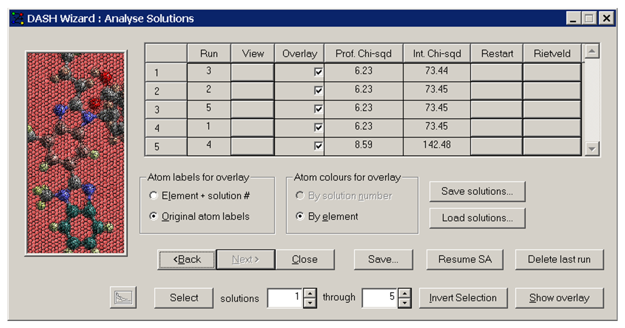
If multiple runs of the SA procedure have been requested (see Simulated Annealing Options), the program will keep a record for each run of the lowest χ² found, and the name of the corresponding solution co-ordinate file. The solution files names are created from the given name of the run with the text suffix _001, _002, … The solutions are sorted into ascending order of Profile Chi-squared in the display:

• Selecting the View button for a specific solution allows you to view the crystal structure and the calculated profile. The overlay check boxes allow you to select the solutions for which the crystal structures are to be shown overlaid in a single unit cell.

• Any of the simulated annealing solutions can be Rietveld refined by clicking the appropriate Rietveld button. Usually, this will only be done for the best solution.

• Save... allows you to save the solutions as .pdb, .cssr, .ccl, .cif, .res and .pro. You can also save the final values of the SA parameters and the χ² progress.

• Save solutions... enables you to save all solutions plus the diffraction pattern and the Pawley fit in one binary file with the extension .dash.

• Load solutions... enables you to load solutions with the extension .dash.

• Resume SA allows you to resume the simulated annealing where it left off. New runs will be appended to the existing one.

• Delete last run: enables you to delete the last solution listed in the summary window. A .dash file saved after solutions have been deleted will not include the solutions deleted.

• Selecting a solution’s Restart button starts the simulated annealing with this solution’s parameters as the initial parameters. The initial parameters are not randomised and existing runs are overwritten.

Reproducibility of Solution

A good indicator is the reproducibility of the structure solution using different starting seeds. If the process keeps converging to the same minimum after multiple simulated annealing runs, you can have increasing confidence in the solution.

Things to Try When Structure Solution Fails

• Review the original data; e.g. do the ESDs look reasonable; have all corrections been applied?

• Review the indexing and the Pawley fit; if necessary, try solving the structure in a different space group.

• Check the molecular stereochemistry, or ring conformation, or whatever else might be relevant. Might there be solvent present and are you sure of the molecular structure?

• Have you frozen any torsion angles around single bonds? If so, consider releasing them.

• Conversely, if the number of parameters is large, try reducing the search space by fixing torsion angles to likely values or, at least, to smaller ranges.

• Try altering the non-hydrogen atom temperature factors.

• Persevere: if the data are reasonably good, Z’=1, and the number of rotatable torsions is < 10, DASH should be able to solve the structure with ease.

Final Rietveld Refinement

• The solution found by DASH may be verified by Rietveld refinement using a program such as TOPAS, GSAS, FullProf or RIETAN. DASH provides an interface to TOPAS, GSAS and RIETAN, though the interface to these 3rd party programs is not actively supported.

• It is also possible to do a rigid-body Rietveld refinement in DASH (see Rietveld Refinement in DASH).

• Initially, try refining only the scale factor and a global temperature factor.

• Following this, if necessary, you can attempt to use highly constrained Rietveld refinement of the atomic positions and isotropic temperature factor and/or refine preferred orientation.

There are a great many packages capable of performing Rietveld refinement of an output structure. Many of these are commercial and are shipped with diffractometers so consult your diffractometer manufacturer for details. There are also several freely available packages, such as DBWS, CCSL, GSAS, and FullProf. A good starting point is to visit http://www.ccp14.ac.uk, where many of the programs can be downloaded, together with examples and tutorials.

DASH Limitations

• Generally, given reasonable data, DASH is routinely successful on structures containing one molecule in the asymmetric unit and up to 10 flexible torsion angles. With more flexible molecules, or with structures containing two molecules in the asymmetric unit, the solution is often found if care is taken.

• Hard limits: 300 atoms, 600 reflections, 15000 data points.

• Although DASH is at the heart of the structure solution process, it is not completely stand-alone. You will need to use some other programs, all of which can be obtained easily and with little or no expense. Specifically, you will need programs for:

• Checking for possible unit cells of higher symmetry (see Appendix B: Programs for Indexing and Cell Reduction).

• Building molecules in 3D (see Appendix C: Programs for Building 3D Molecules).